Multi-visit Mosaic Processing
- Multi-Visit Mosaic (MVM)
A Multi-Visit Mosaic (MVM) is a single image (product) made by combining all observations taken of the same part of the sky.
Observations taken of the same part of the sky over all the years that HST has been operational can enable unique science due to the high-resolution of the HST cameras. Generating useful mosaics from these observations, though, requires solving a number of key problems; namely,
aligning all the images to the same coordinate system
define the size on the sky of each mosaic
defining what exposures should go into each mosaic
MVM processing implemented as part of the Hubble Advanced Products (HAP) pipeline generates new products based on solutions implemented for these critical issues.
Alignment
Generating MVM products relies entirely on the definition of the WCS of each input image in order to define where each exposure will land in the output mosaic. Errors in an input exposure’s WCS will lead to misalignment of overlapping exposures resulting in smeared sources or even multiple images of the overlapping sources in the output mosaic. Errors in the WCS primarily stem from images being aligned to different astrometric catalogs. For example, one exposure may be aligned successfully to the GAIADR2 catalog, yet another overlapping exposure can only be aligned to the 2MASS catalog due to the lack of GAIA sources in the offset exposure.
MVM processing relies entirely on the alignment that can be performed on the exposures during standard pipeline processing and subsequently as part of the Single-Visit Mosaic (SVM) processing. This allows each visit to be aligned to the most accurate catalog available while taking into account the proper motions of the astrometric sources in the field based on the date the exposures were taken in the visit.
By default, the most current GAIA catalog will be used as the default astrometric catalog for aligning all exposures which typically results in images that are aligned well enough to avoid serious misalignment artifacts in the regions of overlap. Unfortunately, due to the nature of some of the fields observed by HST, not all exposures can be aligned to a GAIA-based catalog using GAIA astrometric sources. As a result, the sources used for alignment will have much larger errors on the sky compared to the errors of GAIA astrometric sources which can lead to offsets from the GAIA coordinate system of a significant fraction of an HST pixel (or even multiple HST pixels). This will lead to artifacts in MVM products where such exposures overlap other exposures aligned to other catalogs, especially GAIA-based catalogs.
Defining the Mosaic on the Sky
MVM products need to be defined in order to understand what input exposures will contribute to each mosaic. The solution implemented for HAP MVM products relies on tesselation of the entire sky using the same basic tiles defined by the PanSTARRS project as described at PanSTARRS Sky tessellation patterns.
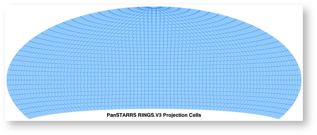
Aitoff plot of all 2,009 PS1 projection cells for the 3PI survey. The coverage extends from declination −30° to the north celestial pole.
PS1 projection cells near the north celestial pole, where the image overlap is greatest due to convergence of the RA grid. The projection cells are 4°x4° in size and are on rings spaced by 4° in declination.
MVM processing uses these pre-defined projection cells after extending them to cover the entire sky with cells that are actually 4.2°x4.2° in size and are on rings spaced by 4° apart in declination. This provides sufficient overlap to allow data from one projection cell to be merged with data from a neighboring cell if necessary. These cells, defined as the ProjectionCell object in the code and referred to as ProjectionCell, are indexed starting at 0 at δ = −90° (South Pole) and ending at 2643 at δ = +90° (North Pole). As stated in the PanSTARRS page:
The projection cell centers are located on lines of constant declination spaced 4° apart. At a given declination, the pointing centers are equally spaced in right ascension around the sky, with the number of RA points changing to account for the convergence of RA lines in the spherical sky. The pattern is defined to cover the entire sky from δ = −90° to +90°… Within a given declination zone, the projection cells are centered at RA(n) = n Δα = n 360°/M where M is the number of RA cells in the zone. Finally, the projection cells themselves are numbered consecutively (ordered by increasing RA) starting at 0 at the south pole, 1–9 at δ = −86°, etc.
All these definitions, including how finely each ProjectionCell should be divided to define the SkyCells, are encoded in a
FITS table installed as part of the drizzlepac package:
drizzlepac/pars/allsky_cells.fits
Defining each SkyCell
Each ProjectionCell is split into a grid of 21 x 21 ‘sky cells’ which serves as the most basic MVM product generated during MVM processing. Sky cells, as defined as the SkyCell object in the code and referred to as SkyCell, are approximately 0.2° x 0.2° in size (~18000 x ~18000 pixels) and they have the same WCS as the ProjectionCell. Each SkyCell gets identified by its position within the ProjectionCell as shown in this figure:
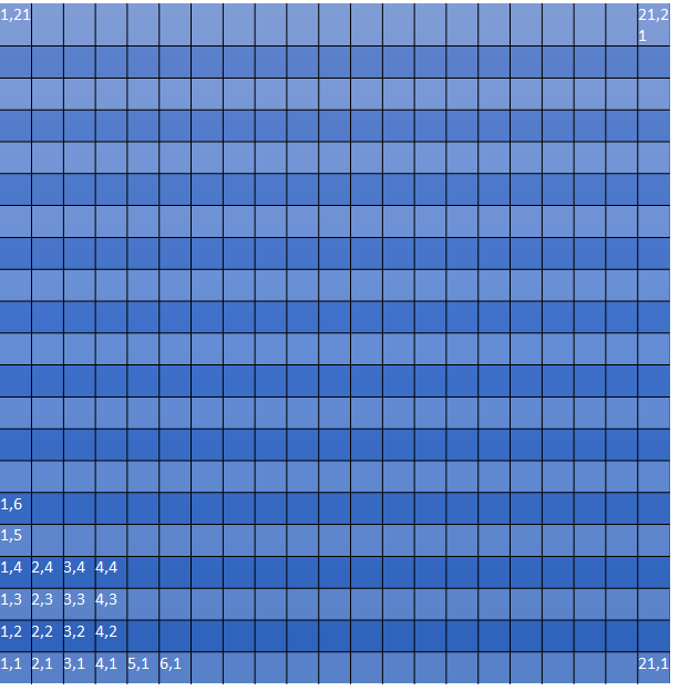
Numbering convention for SkyCells within a Projection Cell used for naming the SkyCell.
The numbering of the SkyCells within a ProjectionCell starts in the lower left corner at (1,1) corresponding to the cell with the lowest declination and largest RA since the SkyCell is oriented so that the Y axis follows a line of RA pointing towards the North Pole. This indexing provides a way to identify uniquely any position on the sky and can be used as the basis for a unique filename for all products generated from the exposures that overlap each SkyCell. Mosaics generated for each SkyCell uses this indexing to create files with names using the convention:
skycell-p<PPPP>x<XX>y<YY>
- where:
Element
Definition
<PPPP>
ProjectionCell ID as a zero-padded 4 digit integer
<XX>,<YY>
SkyCell ID within ProjectionCell as zero-padded 2 digit integers
The WCS for each SkyCell gets defined as a subarray of the Projection cell’s WCS. This allows data across SkyCells in the same ProjectionCell to be combined into larger mosaics as part of the same tangent plane without performing any additional resampling.
Code for Defining SkyCell ID
The code for interfacing with the cell definitions table can be imported in Python using:
from drizzlepac.haputils import cell_utils
Determining what SkyCells overlap any given set of exposures on the sky can be done using the function:
sky_cells_dict = cell_utils.get_sky_cells(visit_input, input_path=None)
where visit_input is the Python list of filenames of FLT/FLC exposures. These files can be any set of FLT/FLC files and the WCS solutions defined in them will, by default, be used as-is to create the final combined mosaics. The MVM products generated in the HST pipeline and stored in the HST archive will be generated using FLT/FLC files that have been aligned to an astrometric catalog like GAIAeDR3 during SVM processing, if alignment was possible at all for the exposure. The full set of parameters that can be used to control the sky cell definitions and IDs can be found in the MVM Processing Code API page.
Exposures in an input list are assumed to be in the current working directory when running the code, unless input_path has been provided which points to the location of the exposures to be processed. The return value sky_cells_dict is a dictionary where the keys are the names (labels) of each overlapping SkyCell and the value is the actual SkyCell object which contains the footprint and WCS (among other details) of the SkyCell.
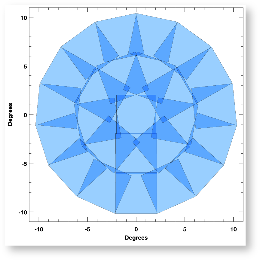
For example, observations from HST proposal 14175 were taken to study NGC 4594 (Sombrero Galaxy) using both the ACS and WFC3 cameras. The footprints of all the HST/ACS and HST/WFC3 observations taken in this part of the sky as shown by MAST can be seen here:
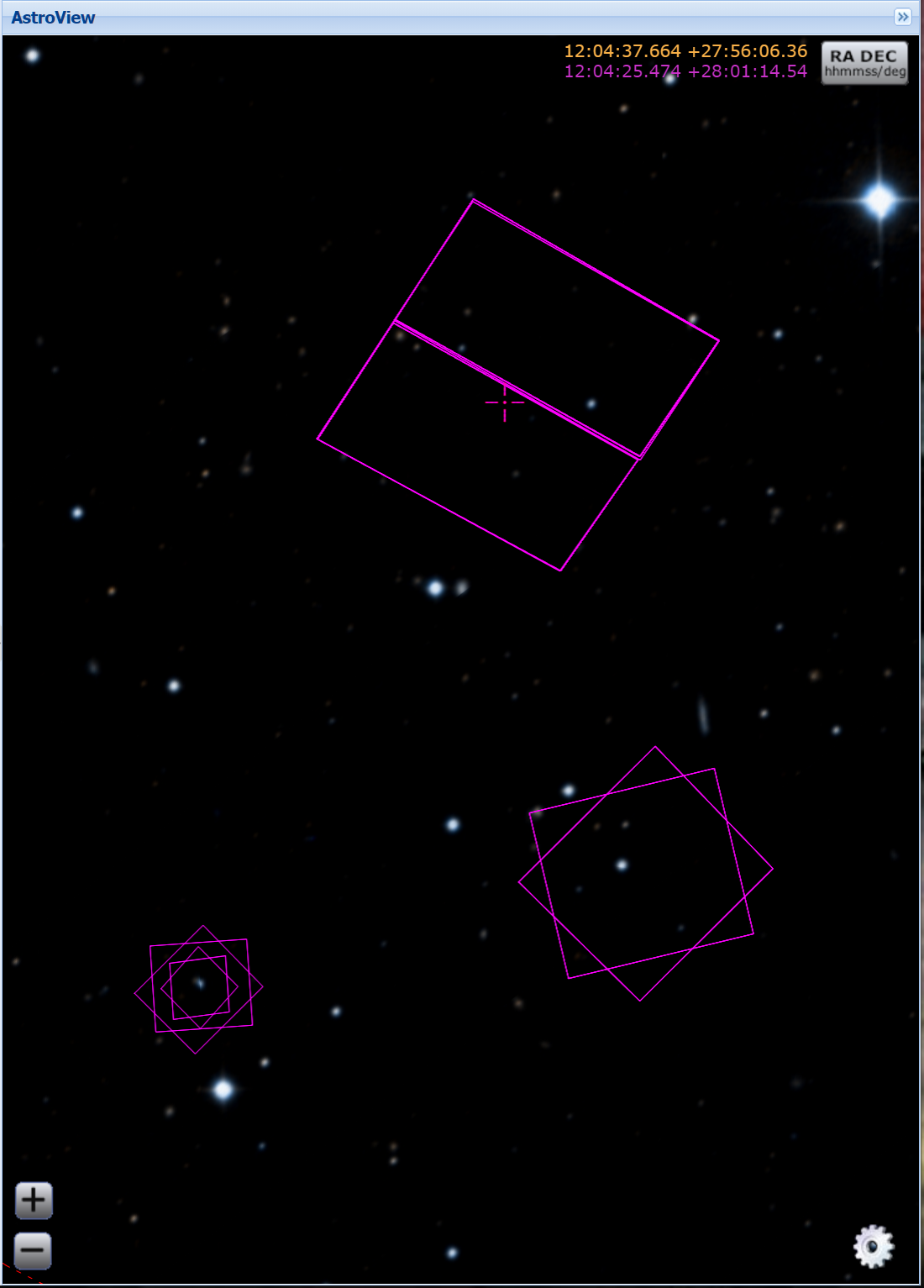
Footprints of HST/ACS and HST/WFC3 observations of the the quasar PG1202+281 and surrounding area.
There were 25 FLT and FLC exposures taken as part of this proposal making up these footprints. The list of these
files defined what was provided as visit_input to the get_sky_cells()
function to get these SkyCell definitions:
sky_cells_dict = cell_utils.get_sky_cells(visit_input, input_path=None)
sky_cells_dict

{'skycell-p1889x07y19': SkyCell object: skycell-p1889x07y19,
 'skycell-p1889x07y20': SkyCell object: skycell-p1889x07y20,
 'skycell-p1970x15y03': SkyCell object: skycell-p1970x15y03,
 'skycell-p1970x15y02': SkyCell object: skycell-p1970x15y02,
 'skycell-p1970x16y02': SkyCell object: skycell-p1970x16y02}
This indicates that these exposures overlap 5 SkyCells in 2 ProjectionCells p1889 and p1970 with the WCS defined in the defined SkyCell object for each SkyCell entry in this dictionary. Each SkyCell object includes a list of all the exposures that overlap just that SkyCell, which can be used to generate those mosaics. Full details of the contents of the SkyCell object can be found in the Multi-visit Processing API documentation.
We can see that one SkyCell includes all exposures using:
for sky_cell in sky_cells_dict:
    print(sky_cell, len(sky_cells_dict[sky_cell].members))

skycell-p1889x07y19 25
skycell-p1889x07y20 8
skycell-p1970x15y03 8
skycell-p1970x15y02 17
skycell-p1970x16y02 8
All subsequent examples will use the exposures for SkyCell skycell-p1889x07y19.
Input Poller File
The MVM processing could simply combine whatever input files are present in the current working directory. However,
that may result in working with more than 1 SkyCell at a time which can, for some steps, end up requiring more memory
or disk space than is available on the system. Therefore, the code relies on an input poller file which specifies exactly
what files should be processed at one time. This ASCII CSV-formatted input poller file will only contain
the names of exposures which
overlap only a single SkyCell regardless of instrument, detector or any other observational configuration.
Generating one of these input ‘poller’ files with the filename skycell-p1889x07y19_mvm_input.txt can be done using the same SkyCell dictionary defined earlier with the commands:
from drizzlepac.haputils import make_poller_files as mpf

with open('skycell-p1889x07y19_input.txt', 'w') as fout:
    _ = [fout.write(f'{sky_cell}\n') for sky_cell in sky_cells_dict['skycell-p1889x07y19'].members]

mpf.generate_poller_file('skycell-p1889x07y19_input.txt',
                         poller_file_type='mvm',
                         output_poller_filename='skycell-p1889x07y19_mvm_poller.txt',
                         skycell_name='skycell-p1889x07y19')
The full description of the function used to create this poller file can be found in the Multi-visit Processing Code API documentation.
This input file skycell-p1889x07y19_mvm_input.txt can then be used as input to the top-level MVM processing code using:
from drizzlepac import hapmultisequencer
rv = hapmultisequencer.run_mvm_processing("skycell-p1889x07y19_mvm_poller.txt")
The poller file contains 1 line for each input exposure for a given SkyCell. The form of the file, though,
is a comma-separated (CSV) formatted file with all the same information as the SVM input files plus a couple of
extra columns; namely,
SkyCell ID
status of MVM processing
An example of an exposure’s line in the poller file would be:
hst_12286_0r_acs_wfc_f775w_jbl70rtv_flc.fits,12286,BL7,0R,486.0,F775W,WFC,skycell-p1889x07y19,NEW,g:\data\mvm\p1889x07y19\hst_12286_0r_acs_wfc_f775w_jbl70rtv_flc.fits
where the elements of each line are defined as:
filename, proposal_id, program_id, obset_id, exptime, filters, detector, skycell-p<PPPP>x<XX>y<YY>, [OLD|NEW], pathname
The SkyCell ID will be included in this input information to allow for grouping of exposures into the same SkyCell layer based on filter, exptime, and year.
The value of ‘NEW’ specifies that this exposure should be considered as never having been combined into this SkyCell’s mosaic before. A value of ‘OLD’ instead allows the code to recognize layers that are unaffected by ‘NEW’ data so that those layers can be left alone and NOT processed again unnecessarily. As such, it can serve as a useful summary of all the input exposures used to generate the mosaics for the SkyCell.
Defining SkyCell Layers
Defining the SkyCell for a region on the sky allows for the identification of all exposures that overlap that WCS. However, creating a single mosaic from data taken with different detectors and filters would not result in a meaningful result. Therefore, the exposures that overlap each SkyCell get grouped based on the detector and filter used to take the exposure to define a ‘layer’ of the SkyCell. Each layer can then be generated as the primary basic image product for each SkyCell. Exposures taken with spectroscopic elements, like grisms and prisms, and exposures taken of moving targets can not be used to create layers due to the inability to align them with the rest of the observations. Therefore, only images taken with standard filters (like the WFC3/UVIS F275W filter) will be used to define SkyCell mosaics (layers).
The default plate scale for all MVM image products for each SkyCell has been defined as 0.04”/pixel to match the higher resolution imaging performed by the WFC3/UVIS detector. However, WFC3/IR data suffers from serious resampling artifacts when drizzling IR data to that plate scale. So in addition to creating IR mosaics at the 0.04”/pixel ‘fine’ plate scale, IR mosaics are also generated at a ‘coarse’ plate scale of 0.12”/pixel to minimize the resampling artifacts while also being easily scaled to the ‘fine’ plate scale mosaics.
SkyCell Layers Example
For example, observations were taken with Proposals 12286 and 12903 using both the ACS and WFC3 cameras and multiple filters. The ACS observations were taken with the ACS/WFC detector using the F775W and F850LP filters, while the WFC3 observations were taken using the IR detector using the F105W, F125W and F160W filters as well as the UVIS detector using the F475W. All these observations fall within the SkyCell at position x07y19 in the ProjectionCell p1889, but given the dramatic plate scale differences, these observations can not be used to create a single mosaic.
The different observing modes used for observations in this SkyCell end up being organized as 9 separate layers (mosaics); namely,
wfc3_uvis_f475w (0.04”/pixel)
wfc3_ir_f105w_coarse (0.12”/pixel)
wfc3_ir_f105w (0.04”/pixel)
wfc3_ir_f125w_coarse (0.12”/pixel)
wfc3_ir_f125w (0.04”/pixel)
wfc3_ir_f160w_coarse (0.12”/pixel)
wfc3_ir_f160w (0.04”/pixel)
acs_wfc_f850lp (0.04”/pixel)
acs_wfc_f775w (0.04”/pixel)
Since they all have the same WCS, modulo the plate scale differences, they can be overlaid pixel-by-pixel with each other for analysis.
You can verify this interactively by directly calling the code that interprets the input ‘poller’ file using:
from drizzlepac.haputils import poller_utils

obs_dict, tdp_list = poller_utils.interpret_mvm_input('skycell-p1889x07y19_mvm_poller.txt',
                                                      log_level=poller_utils.logutil.logging.INFO)
for layer in obs_dict:
    print(obs_dict[layer]['info'])

skycell-p1889x07y19 wfc3 uvis f475w all all 1 drz fine
skycell-p1889x07y19 wfc3 ir f105w all all 1 drz coarse
skycell-p1889x07y19 wfc3 ir f105w all all 1 drz fine
skycell-p1889x07y19 wfc3 ir f125w all all 1 drz coarse
skycell-p1889x07y19 wfc3 ir f125w all all 1 drz fine
skycell-p1889x07y19 wfc3 ir f160w all all 1 drz coarse
skycell-p1889x07y19 wfc3 ir f160w all all 1 drz fine
skycell-p1889x07y19 acs wfc f850lp all all 1 drc fine
skycell-p1889x07y19 acs wfc f775w all all 1 drc fine

print(tdp_list)

[<drizzlepac.haputils.product.SkyCellProduct at 0x1fd04dcc220>,
 <drizzlepac.haputils.product.SkyCellProduct at 0x1fd04d49a60>,
 <drizzlepac.haputils.product.SkyCellProduct at 0x1fd04d49cd0>,
 <drizzlepac.haputils.product.SkyCellProduct at 0x1fd04dccd30>,
 <drizzlepac.haputils.product.SkyCellProduct at 0x1fd04dcc0a0>,
 <drizzlepac.haputils.product.SkyCellProduct at 0x1fd04dccfd0>,
 <drizzlepac.haputils.product.SkyCellProduct at 0x1fd04dcca60>,
 <drizzlepac.haputils.product.SkyCellProduct at 0x1fd117a1e50>,
 <drizzlepac.haputils.product.SkyCellProduct at 0x1fd04d53910>]
These objects define the WCS, inputs and filenames for each layer for use in creating these products. Full details of the contents of the SkyCellProduct can be found in Multi-visit Processing Code API documentation.
MVM Processing Steps
The definitions for the ProjectionCell and SkyCell allow for all HST observations to be processed into a logical set of image mosaic products regardless of how many observations cover any particular spot on the sky while tying them all together in the same astrometric reference frame (as much as possible, anyway). The steps taken to generate these MVM products can be summarized as:
Determine what SkyCell or set of SkyCells each exposure overlaps
Copy all relevant exposures for a given SkyCell into a single directory for that SkyCell
Rename input exposures to have MVM-specific filenames
Generate input file to be used for processing each SkyCell
Evaluate all input exposures to define all layers needed for the SkyCell
Determine which layer to process
Drizzle all exposures for each layer to be processed to create new mosaic product for that layer
Running MVM Processing
The primary function used to perform MVM processing interactively in a Python session is:
from drizzlepac import hapmultisequencer
r = hapmultisequencer.run_mvm_processing(input_filename)
The function takes several optional parameters to control aspects of the processing, with full details of this function’s parameters and all related functions being described in Multi-visit Processing API.
SkyCell Membership
Data from HST gets organized based on a filename derived from the proposal used to define the observations and how
HST should take them. MVM processing, on the other hand, focuses on how the observations relate to each other on the
sky based on the WCS information. The cell_utils module includes the code used to interpret
the WCS information for exposures and determine what ProjectionCells and SkyCells each exposure overlaps as shown in the
section on the Code for Defining SkyCell ID.
This code can be called on any set of user-defined exposures to determine for the first time what SkyCells the exposures overlap. During HST pipeline processing, this code gets called for the exposures from each visit after they have finished SVM processing and after they have been aligned as much as possible to the latest astrometric reference frame (such as the GAIAeDR3 catalog). Using these updated WCS solutions provides the most accurate placement of the exposures on the sky and therefore in the correct SkyCell.
Copy Data
The MVM processing code requires the input exposures to be located in the current working directory as the processing may require the ability to update the input files with the results of the MVM processing. Each input file may also overlap more than 1 SkyCell. As a result, the input files get copied into a directory set up specifically for processing a given SkyCell. This results in each input file being copied into as many directories as needed to support creating the mosaics for as many SkyCells as desired while protecting the integrity of the original input files and their WCS solutions.
Rename Input Files
The MVM processing code works on the input files provided using the WCS solutions defined in the headers of the input files as-is for the initial implementation. However, in order to preserve the solutions defined by previous processing steps, these files are renamed based on the SkyCell to be generated in the current working directory.
For reference, the original pipeline-assigned name has the format of:
IPPPSSOOT_flc.fits
- such as
jcz906dvq_flc.fits
icz901wpq_flc.fits
The MVM filename defined for the input exposures follows the convention.
hst_skycell-p<PPPP>x<XX>y<YY>_<instr>_<detector>_<filter>_<ipppssoo>_fl[ct].fits
- where:
Element
Definition
<PPPP>
ProjectionCell ID as a zero-padded 4 digit integer
<XX>,<YY>
SkyCell ID within ProjectionCell as zero-padded 2 digit integers
<instr>
Name of HST instrument from INSTRUME header keyword
<detector>
Name of detector from DETECTOR header keyword
<filter>
Name of filter from FILTER or FILTER1,FILTER2 header keyword(s)
<ipppssoo>
Pipeline-assigned IPPPSSOO designation from original input filename
fl[ct]
Suffix of either flt or flc from original input filename
This insures that each exposure gets renamed in a way that allows them to be easily identified with respect to the output SkyCell layer the exposure contributes to during MVM processing.
Note
The currently implemented MVM processing does not update the WCS and DQ arrays of these input files in any way. As a result, they only get used as intermediate products, and get deleted automatically upon successful completion of MVM processing. Should future updates to MVM processing be implemented, for example to further refine the alignment, then these products would get updated at that time and be added as a new product to the HST archive instead of being deleted.
Primary MVM Processing Interface
MVM processing gets controlled through a single function:
from drizzlepac import runmultihap

rv = runmultihap.process(input_filename)
This function takes as either form of the input file generated for the input exposures in the current directory
as the input parameter input_filename. This function then performs all the processing steps automatically to
generate the image mosaics from the exposures listed in the input file.
There are times, though, when the default processing needs to be revised to account for the science goals of the processing or to account for the exposures available as inputs. The following environmental variables can be used to control how the MVM processing deals with various types of input files:
- MVM_INCLUDE_SMALL
This controls whether or not layers are created for ACS/HRC or ACS/SBC exposures given their small field-of-view. By default, this is turned on (‘true’) so that these layers are created.
- MVM_ONLY_CTE
This controls whether or not to include exposures which have NOT been CTE-corrected due to the potential impact to the output mosaics PSFs from including exposures with CTE tails. By default, this is actually turned off (‘false’) so that all data gets used.
These variables can be set to values of ‘on’, ‘off’, ‘true’, ‘false’, ‘yes’ or ‘no’ in the operating system environment
or even in the python environment using os.environ.
Additionally, the function run_mvm_processing(), which gets called by
perform(),
has the ability to enable an additional attempt to align all the
input exposures to the latest astrometric catalog, as well as limit the size of the output mosaics.
Full details of these parameters are available in the discussion of the
Multi-visit Processing Code API documentation.
Define SkyCell Layers
SkyCells define the WCS that will be used for all the observations for any given region on the sky. However, it doesn’t make sense to create a single image from all the exposures due to differences in the detectors, pixel sizes, PSFs and filters used for the observations. It can even be argued that observations taken too far apart in time should also not be combined, or observations taken with dramatic differences in exposure time should not be combined. As a result, the concept of a SkyCell ‘layer’ was implemented to organize all the exposures for a SkyCell into sets of exposures which can be combined to create useful, and hopefully scientifically interesting, mosaics.
The most basic definition for a layer organizes the exposures based on the following criteria:
instrument
detector
filter
Using the renamed input files, the MVM processing code organizes all the exposures based on these criteria to identify what layers could be generated from all the inputs. For example, a SkyCell with ACS/WFC3 F814W exposures and WFC3/UVIS F606W exposures would result in 2 SkyCell layers being defined; namely, one for each set of exposures.
Note
Observations taken with a spectroscopic element, like grisms or prisms, will not be used to define SkyCell layers.
Determine Layers to Process
Specifying what input exposures need to be used to create a SkyCell layer mosaic serves as a critical feature of the
input file. Input files simply listing filenames indicate that ALL exposures specified should be used to create MVM
products. However, the more descriptive poller file CSV format input file provides the ability to limit the processing
to only new exposures, while treating already archived versions of the MVM products for all the other SkyCell layers as
fully updated and not in need of any further processing. This control comes from the entry that specifies ‘NEW’ or ‘OLD’,
with only those layers with at least 1 ‘NEW’ entry getting defined for processing.
Create SkyCell Mosaics
The input files get interpreted to define the image products that need to be created when combining the exposures. These mosaics get generated by drizzling the input exposures onto the WCS defined for the SkyCell, creating a separate mosaic for each layer from all the exposures with the same filter/detector/instrument configuration.
The drizzle parameters used to create these products are determined based on the average number of exposures for all the exposed pixels in the SkyCell layer. This only serves as an approximation of what would work best across the entire SkyCell layer, as some portions may only have a single exposure while other regions may have many overlapping exposures. However, this still works reasonably well due to the fact that only the following drizzle steps are actually applied when creating the MVM products:
sky matching
final drizzling with bad pixel rejection
These products, thus, rely entirely on the DQ arrays to be updated by SVM and pipeline processing to flag cosmic-rays and detector artifacts as bad pixels so those pixels get rejected when creating the MVM product. In addition, they rely on the WCS solutions provided by previous processing as well to place the exposures in the final MVM product.
The parameters used for creating these drizzle products can be found installed with the package’s code. You can find the files using:
import os
import drizzlepac
#
# Directory is:  drizzlepac/pars/hap_pars/mvm_parameters
#
os.chdir(os.path.join(drizzlepac.__path__, 'pars', 'hap_pars', 'mvm_parameters'))
There are separate configuration files for each detector based on the number of average exposures in the output frame.
The final output products get created with a final output array size that is trimmed down to only the subsection of the entire SkyCell which has HST data in any layer.
Finally, the output drizzle product will have a filename that follows the basic convention used to rename the input exposures without the final ‘ipppssoo’ designation; namely,
hst_skycell-p<PPPP>x<XX>y<YY>_<instr>_<detector>_<filter>_<layer>_dr[cz].fits
- where:
Element
Definition
<PPPP>
ProjectionCell ID as a zero-padded 4 digit integer
<XX>,<YY>
SkyCell ID within ProjectionCell as zero-padded 2 digit integers
<instr>
Name of HST instrument from INSTRUME header keyword
<detector>
Name of detector from DETECTOR header keyword
<filter>
Name of filter from FILTER or FILTER1,FILTER2 header keyword(s)
<layer>
Layer-specific designation: coarse-all or all
dr[cz]
Suffix of either DRZ or DRC based on input filenames
The <layer> component of the MVM filename indicates the plate scale and any other criteria used to define the layer such as exposure time or date range of exposures used to create the layer. At present, only WFC3/IR data gets generated with both the default (fine) plate-scale of 0.04”/pixel as well as the IR-native “coarse” plate scale which show up with a <layer> term of coarse-all. Initial processing does not apply any additional definitions for the layers, and thus the remainder of the initially generated MVM products simply have a <layer> term of all. Future processing may enable generation of additional layers based on date ranges for SkyCells which have massive amount of exposures over a large range of dates, in which case this <layer> term will be updated to reflect those ranges. Additionally, the code can be run interactively to enable generation of additional layers based on exposure time ranges as well. See explanation of the processing code functions for more details.